Optimum Machine Design

Here are some materials that are intended to help with transferring existing TK Solver code into modeFrontier. This is done in order to utilize the wide variety of optimization and data analysis tools that modeFrontier offers. It also serves as a starting point for any further work on integrating modeFrontier with the full complement of software used the University of Idaho Mechanical Engineering Department.

Workflow: TK Solver à Excel à modeFrontier

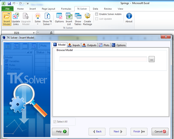
The basis of the optimization work that follows is a workflow that was developed for a Capstone Design project involving engine design, but is broadly applicable to any program that can be written in TK Solver. In this example the optimization of a compression spring for the minimization weight is being performed. The first step in this process is exporting the TK Solver code into Excel. This is done in Excel through the TK Solver tab located at the top of the interface. Then, after clicking the insert model button the interface shown below will appear.

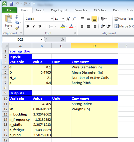
In this interface the proper TK Solver model is selected, and any input and output variables pertinent to the desired optimization process are selected. This will then generate an Excel spreadsheet that will perform the same function as the underlying model. This sheet will update after every change to values in the input cells. An example of this Excel spreadsheet is shown here.

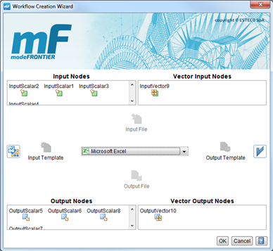
Once the Excel workbook has been tested to verify that it works correctly the process of building the modeFrontier workflow can begin. Upon starting modeFrontier you will be given the option to create a new project. This will create a blank page where any workflow can be created. For new users there is also a better option available that is to use the Workflow Wizard. This allows the user to quickly select inputs, outputs, and what software you would like to interface with. After clicking OK a generic workflow will appear. This workflow needs to be further customized for ease of use and functionality. To aid in understanding of your workflow it is helpful to rename the inputs and outputs to their names in the original TK Solver code. Things such as constraints, goals, DOEs, and Schedulers must also be selected, and are covered in more detail in the appropriate section. Below is the example of the finished workflow for the compression spring mass reduction problem.

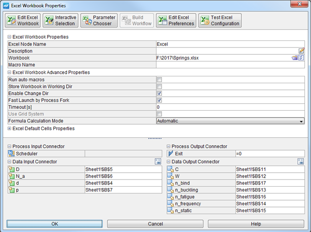
The final step for this setup is to properly configure the interface between mode frontier and Excel. This is done by clicking on the Excel node in the workflow. This will bring up the following interface where you should first locate the correct workbook, and then properly input the correct cell locations alongside the corresponding variables. Be very careful to follow the format for cell locations exactly as shown below. Even if the workbook contains only one sheet you must still clarify that the location is on sheet one otherwise the input/output connection will not work properly.

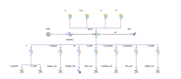
Once these steps have all been completed the model should run any designs given by the DOE and scheduler. However, this is not enough information to properly run an optimization. To optimize the design objectives and constraints must first be configured.

Objectives and Constraints

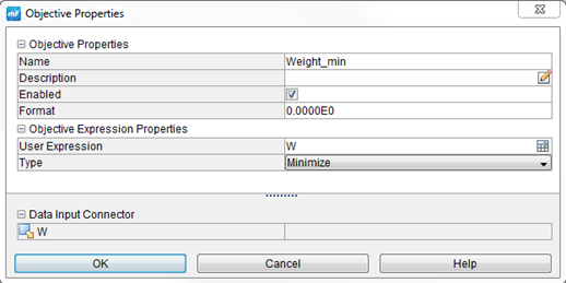
In modeFrontier there are multiple types of objectives that each have unique purposes. The most common is simply called the objective. It can be either the minimization or maximization of any function that the user inputs. This function is entered in the user expression field, and must be written with proper JavaScript syntax. This function is often just the name of an output variable as is in the case shown where the weight calculated by TK Solver is being minimized. The other type of objective that is commonly utilized is the target value objective. When a target node is connected to an output variable you can enter a target value that the optimization will attempt to reach. There are also other types of objectives available for handling vectors and other datatypes. More information on these can be found in the modeFrontier user manual.

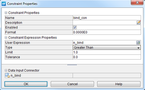
Sometimes it is useful to only look at data that meets certain prescribed conditions. For example, in the spring design problem given it would not make sense to consider designs that have safety factors of less than one. The springs index must also be limited to a narrow range of acceptable values. In both these cases the way to impose this limitation is with a constraint. This constraint can be of greater than, equal to, or less than types, and like the objectives accept any valid JavaScript expression. Constraints are only used on outputs, if an input can only be within a certain range then that range can simply be set in the input properties, and no designs outside that range will be created. On the other hand, with a constrained output some designs will be generated that fail to satisfy the constraint. In this case the designs will be labeled as invalid, and the optimization algorithm will impose a penalty to direct the generation of further designs away from those that violate the constraint.

DOE and Scheduler

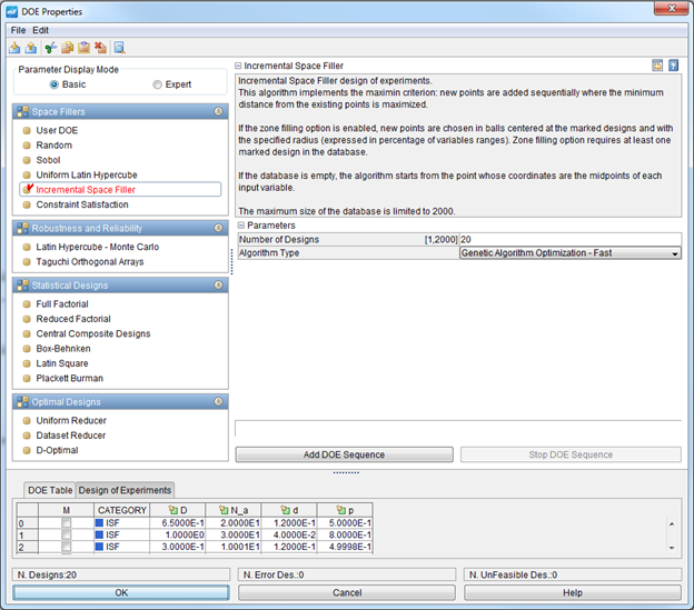
In modeFrontier both the DOE and Scheduler determine which designs will be evaluated. The DOE provides the initial designs that will be evaluated, and then the responses of those designs will be assessed by the scheduler to generate new designs according to the chosen optimization algorithm. The various types of DOEs available are shown below.

Unless the user is aware of where in the design space the optimal design is located it is best to generate designs that are distributed throughout the entire design space. These are broadly classified as space filler DOEs. If each iteration of the problem is solved quickly then many data points can be evaluated in a short amount of time. In this case random generating of the DOE is acceptable, as the number of points generated should be high enough that no clusters of points are apparent. If evaluating a large number of designs is too time consuming, then the Incremental Space Filler or Uniform Latin Hypercube DOEs will ensure that the designs are well distributed through the design space. 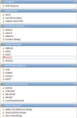Finally, if you do have a known good design to start from you can add it using the User DOE option.

The Scheduler in modeFrontier is the optimization algorithm. The options available are shown below, and the most commonly used types are in the Evolutionary, Heuristic, Gradient-Based, Multi-Strategy categories. When to use each type of algorithm is a complex subject that cannot be covered in this quick overview. Documentation for each algorithm is provided in the user manual, and for several algorithms research papers are provided. In general, it is enough to know that a gradient-based algorithm will arrive at the answer quicker, but will sometimes get stuck on a suboptimal design. 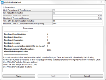In problems that are poorly defined or have statistical variance in their output heuristic and evolutionary algorithms generally perform better.

At the top of the scheduler interface an optimization wizard is provided that will help you determine the best algorithm to select based primarily around the acceptable simulation time. This should provide a good starting suggestion for most well-defined engineering problems.

Data and Analysis

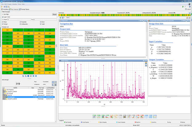
Once the workflow is properly setup it can be run from the Run Analysis tab of the interface. An example of the output from a particle swarm optimization for the compression spring weight minimization problem is shown. In this case 1000 design evaluations were performed, and while several good designs were quickly found the algorithm continued to explore the design space resulting in unacceptable designs at all stages of the process. This is a characteristic of all heuristic algorithms. A gradient based optimization of this problem was also performed, and given the simple nature of the problem it was able to find the optimal design with only 100 design evaluations.

On the left one of the simplest methods for evaluating the outputs of this run has been performed. The data is sorted by the goal function, in this case weight, and then the first design that did not violate the constraints is selected as the chosen design. In a simple optimization such as this which only has one objective this is often the easiest way to evaluate which design is best. When the number of objectives increases it is often better to use a more sophisticated method.

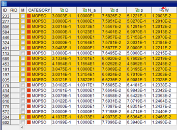
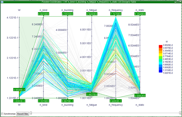
One of the more intuitive ways to sort through designs that works well with multiple objectives is the Parallel Coordinates Chart. This chart traces designs through the corresponding variables, and then allows a filter to be applied to each variable. This allows the user to decide which designs are acceptable, and by selecting any of the curves the exact run number can be determined. Other methods for design selection are included in modeFrontier such as Multi-Criteria Decision Makers which evaluate designs based on weights assigned to each objective. These are suitable when the importance of each design aspect is known, but this is often not the case. Because of this a graphical method such as the Parallel Coordinates Chart or a pareto frontier displayed on a graph for two and three-dimensional problems is often preferred.

Best Practices

The process of creating optimum designs is not always as simple as throwing a large amount of computing power at the problem. Often an answer will be found quicker and easier if more thought is put into the problem formulation. More thought on the side of problem formulation also makes results easier to interpret and design objectives for. One example of this is that it is often easier to create safety factors for all aspects of the design. With this approach all constraints are simply become that the safety factors must be greater than one.

Observation of the outputs form your model is critical to figure out if it is running properly and to determine whether it will converge to an optimum design. A good understanding of the underlying principles is necessary so that the desired outputs can be predicted. If the model does not perform as expected double check the configuration of the objectives and the interface with any external solvers as this is often the source of errors.

If an evolutionary or heuristic algorithm is used multiple designs can be evaluated simultaneously. This option is available in the run options for the scheduler. For these types of algorithms set the number of concurrent designs equal to the number of physical processor cores that the computer has. This will greatly increase to number of designs that can be evaluated within a given time.

Finally, this is only a short guide and cannot provide solutions for all possible issues. It is in the best interest of all users to read every section of the manual pertaining to the type of work that the are undertaking.